Fractional space

All three spatial operators are external UFL operators. Build one and use it as an ordinary term.

The three spatial operators are not interchangeable

SpectralFractionalLaplacian raises the eigenvalues of a chosen Dirichlet operator,

\[ (-\Delta_D)^su=\sum_k\lambda_k^s(u,q_k)q_k, \]

while RieszFractionalLaplacian applies the whole-space singular integral to the zero extension,

\[ C_{2,s}\operatorname{PV}\int_{\mathbb R^2} \frac{u(x)-u(y)}{|x-y|^{2+2s}}\,dy . \]

PeriodicFractionalLaplacian acts on a flat periodic cell through the Fourier-series multiplier

\[ \widehat{(-\Delta_{\mathrm{per}})^s u}_k=|k_L|^{2s}\widehat u_k, \qquad k_L=2\pi(k_1/L_1,\ldots,k_d/L_d). \]

The three realizations have different domains, eigenfunctions, boundary behaviour, numerical parameters, and solvers. A homogeneous trace does not make the Dirichlet and zero-exterior realizations agree. Periodically tiling a field changes the problem again.

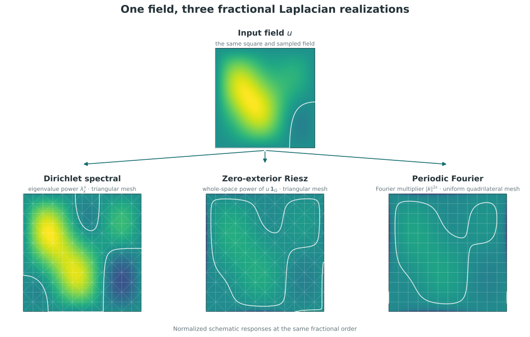
The same field on the same square produces three different responses. The Dirichlet spectral and zero-exterior Riesz realizations are shown on triangular meshes. The periodic Fourier realization is shown on the uniform quadrilateral periodic mesh required by its discrete Fourier transform.

Spectral, homogeneous Dirichlet

Pass the homogeneous boundary condition explicitly:

Lu = SpectralFractionalLaplacian(
    u,
    0.4,
    bcs=bc,
    sinc_truncation_target=1.0e-6,
    shift_cache="all",
)
F = inner(CaputoDerivative(u, alpha), v) * dx + inner(Lu, v) * dx

spectral_fractional_diffusion.py uses a square eigenfunction. spectral_unit_square.py checks the bare action against a known eigenpair. Tighten sinc_truncation_target on a fixed mesh before measuring finite-element convergence, and inspect Lu.diagnostics() for node count and shifted-solver reuse.

Use shift_cache="all" for repeated small problems and "stream" for bounded storage.

Riesz, zero exterior

For \(s<1/2\) no boundary trace is required:

Lu = RieszFractionalLaplacian(u, 0.3)

This uses quadrature_degree=6, the edge rule, and the matrix-free backend. The function is extended by zero outside the polygonal domain.

Limits worth knowing before you build a mesh: scalar CG1 or CG2 only, affine 2D triangles only, and periodic or overlapping geometries are rejected. For \(s\geq1/2\), pass complete homogeneous bcs. A nonzero trace has infinite zero-extension energy.

riesz_fractional_diffusion.py couples it to a Caputo derivative. riesz_zero_exterior.py shows the bare action.

For larger problems, switch the backend and refine compression separately from quadrature:

Lu = RieszFractionalLaplacian(
    u, 0.3, bcs=bc, assembly="hmatrix", compression_tolerance=1e-8,
)

Backend trade-offs are tabulated in Riesz/restricted fractional Laplacian.

Periodic Fourier

Use a fully periodic uniform interval, quadrilateral rectangle, or hexahedral box:

mesh = PeriodicRectangleMesh(
    32, 24, 2*pi, 2*pi, quadrilateral=True, reorder=False,
)
V = FunctionSpace(mesh, "Q", 1)
u = Function(V)
Lu = PeriodicFractionalLaplacian(u, 0.4)

The three-dimensional construction uses the same operator:

mesh = PeriodicBoxMesh(
    24, 20, 16, 2*pi, 2*pi, 2*pi,
    hexahedral=True, reorder=False,
)
V = FunctionSpace(mesh, "Q", 1)
Lu = PeriodicFractionalLaplacian(Function(V), 0.62)

There are no boundary conditions or quadrature controls. Construction checks that the field has exactly one scalar degree of freedom at each periodic grid point and rejects a mesh that is nonuniform, only periodic in one direction, triangular, deformed, or higher order.

periodic_fourier.py applies the operator to \(\sin(2x)\cos(3y)\), whose eigenvalue is \(13^s\). visual_periodic_fractional_gyroid.py evolves the same multiscale three-dimensional periodic field at two fractional orders and renders synchronized zero isosurfaces and midplane slices. The MPI backend supports the full 3D calculation. See Periodic Fourier fractional Laplacian for the exact scope.